Visual Calculations: Introducing a Two-Layer Approach in DAX Calculations

The February release of Microsoft Power BI Desktop unveiled the public preview of a transformative DAX feature – visual calculations. This new feature promises to revolutionize the way calculations are written, making them more intuitive and user-friendly than ever before. As we unpack the layers of this innovation, we’ll discover how it simplifies the creation of dynamic and complex reports, empowers users of all skill levels, and addresses some of the most persistent challenges in data modeling. Given the breadth and depth of this subject, a series of articles is required to sufficiently cover it. In this first article, we begin by exploring one of the motivations for the introduction of visual calculations.

Before the introduction of visual calculations, Power BI users primarily relied on measures to perform calculations within their reports. Measures are a fundamental and distinctive feature offered by Power BI, and they are the primary reason DAX was invented. The power of measures lies in their reusability – you can write a formula once and save it in the semantic model. Then, report creators can simply drag and drop it onto any visual in any report, and it will just work, even in reports you never anticipated initially. This capability is not available with SQL or Python, at least not yet. Although there is a proposal to introduce measures to SQL, it remains just a proposal for now. For the magic of reusability to work, every measure must be independent. For example, [measure 2] = IF([measure 1] > 1000, [measure 1]) means that [measure 2] can calculate [measure 1] internally by itself, without requiring [measure 1] to be added to the same report first. This is convenient and impressive, but what if users also include [measure 1] on the same report? In that case, will [measure 2] be able to take advantage of the values of [measure 1] that are already calculated? Unfortunately, the answer is “it depends,” and it is complicated.

The independent nature of DAX measures can initially surprise users accustomed to other reporting tools, contributing to a significant learning curve for DAX beginners. For example, consider a simple report that includes both the sum of sales and the sum of quantity. A SQL user might typically expect the underlying query to resemble:

SELECT SUM("SalesAmount"), SUM("OrderQuantity") FROM "FactInternetSales"

However, in the DAX world, assuming there are two DAX measures in a DirectQuery model:

[Total Sales] = SUM('FactInternetSales'[SalesAmount])
[Total Quantity] = SUM('FactInternetSales'[OrderQuantity])

This setup would lead to two separate SQL queries if the DAX Engine were to evaluate each measure independently:

SELECT SUM("SalesAmount") FROM "FactInternetSales"
SELECT SUM("OrderQuantity") FROM "FactInternetSales"

It may be surprising to DAX newcomers that even straightforward measures like these could be costly to evaluate if the DAX Engine had adopted a naive execution plan. To reduce redundant calculations, the DAX Engine uses a technology known as fusion, which combines leaf-level calculations into fewer queries to the underlying storage engine, thus optimizing performance. For a visual representation of how fusion optimizes calculations in the DAX Engine, refer to Figure 1. Returning to our earlier example, even if a user includes both [measure 1] and [measure 2] in the same visual, the DAX Engine does not reuse the results of [measure 1] when calculating [measure 2]. Instead, [measure 2] calculates [measure 1] independently. During this process, the leaf-level nodes of [measure 2] might either access the Vertipaq engine cache if [measure 1] has already been calculated, or they may benefit from the fusion optimization to consolidate with the leaf-level nodes of [measure 1].

Figure 1. Fusion Optimization in DAX Queries

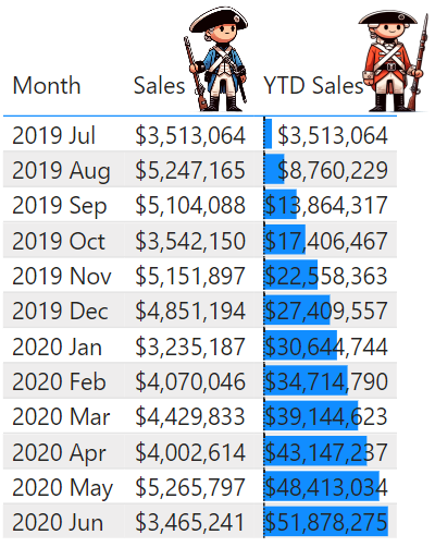
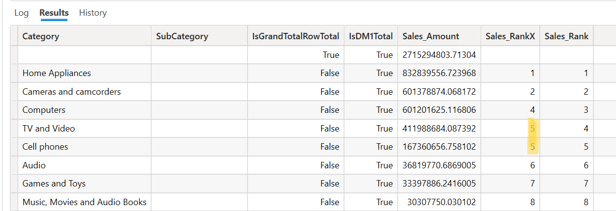
In this article, we will not explore further into the territory of fusion. The mention here serves merely to illustrate the extensive engineering efforts that have been poured into the DAX query optimizer to avoid the prohibitively expensive naive execution plans. The remarkable reusability of DAX measures stems from their design principle of logical independence, which, while seemingly straightforward, requires complex execution plans to merge separate calculations into consolidated operations. Let’s examine a case where this independence leads to suboptimal execution. Refer to Figure 2, which shows a table visual with [Sales] measure values for each month in a fiscal year next to the [YTD Sales] measure, representing the cumulative sums from the beginning to the end of that period. It might seem logical that the [YTD Sales] values could be derived by summing the monthly [Sales] data. However, closer scrutiny reveals that each measure is computed separately. To demonstrate this, four VertiPaq SE Query End events were captured and presented beneath Figure 2, each corresponding to a storage engine query invoked by the DAX query for this visual. Without explaining the specific functions of each storage engine query, it is obvious that the [YTD Sales] measure was calculated independently, resulting in its own set of queries to the Vertipaq Engine.

⚠ For a hands-on experience with the examples used to create Figures 2 and 4, you can download the corresponding pbix from the following link: Download pbix file.

Figure 2. Independence of Measures within a Single Visual

-- Q1
SELECT [Date].[Month], [Date].[MonthKey]
FROM [Date]
WHERE [Date].[Fiscal Year] = 'FY2020';
-- Q2
SELECT [Date].[Date Value], [Date].[Month], [Date].[MonthKey]
FROM [Date]
WHERE [Date].[Fiscal Year] = 'FY2020';	
-- Q3
SELECT [Date].[Date Value], SUM([Internet Sales].[SalesAmount])
FROM [Internet Sales] LEFT OUTER JOIN [Date] ON [Internet Sales].[OrderDateKey]=[Date].[DateKey]
WHERE [Date].[Date Value] IN (43666.000000, 43707.000000, 43748.000000, 43789.000000, 43830.000000, 43871.000000, 43680.000000, 43721.000000, 43762.000000, 43803.000000...[366 total values, not all displayed]);
-- Q4
SELECT [Date].[Month], [Date].[MonthKey], SUM([Internet Sales].[SalesAmount])
FROM [Internet Sales] LEFT OUTER JOIN [Date] ON [Internet Sales].[OrderDateKey]=[Date].[DateKey]
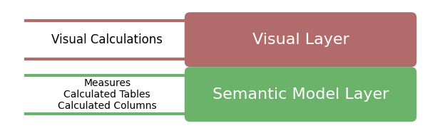
WHERE [Date].[Fiscal Year] = 'FY2020';

Although the DAX Engine development team will continue to create new algorithms to enhance calculation performance, it is impractical to expect them to cover the vast and rapidly growing diversity of DAX expressions in use globally. Similarly, it is unrealistic to expect that every user will achieve expert-level proficiency in row contexts and filter contexts, and thus be able to craft perfectly optimized formulas in all situations. To address this challenge, visual calculations were conceived as a new method for defining calculations directly on top of filtered and aggregated data, thereby completely avoiding the possibility of accidental, expensive scans on physical tables. These visual calculations exist exclusively within the visual layer, separate from the measures located in the semantic model layer, as depicted in Figure 3. This segregation ensures that DAX calculations at each layer have access only to objects within their own layer, allowing authors to immediately determine whether their calculations are interacting with raw data in physical tables or operating solely on filtered and aggregated data. This delineation simplifies the design process, rendering it more intuitive and less prone to errors for users of all skill levels.

Figure 3. Two Layers of Calculations: Visual Layer vs. Semantic Model Layer

Returning to the earlier example of the two measures as shown in Figure 2, I replaced the [YTD Sales] measure with an equivalent visual calculation and achieved the same results, which are displayed in Figure 4. This change resulted in only a single VertiPaq SE Query End event, copied below the figure. ⚠ As visual calculations are still in public preview, some functionalities like number formatting and conditional formatting on the fields are not yet available. These limitations will be lifted before the feature is released for general availability.

Figure 4. Dependence of Visual Calculation on Measure Results

SELECT [Date].[Month], [Date].[MonthKey], SUM([Internet Sales].[SalesAmount])
FROM [Internet Sales] LEFT OUTER JOIN [Date] ON [Internet Sales].[OrderDateKey]=[Date].[DateKey]
WHERE [Date].[Fiscal Year] = 'FY2020';

In this article, we have taken a first look of a new layer of calculation and examined one of the motivations for its development. We have discovered that the reusability of DAX measures originates from their logical independence, which necessitates complex execution strategies to reduce redundant and inefficient calculations. Consequently, this can pose a significant challenge for DAX measure authors to craft efficient calculations that satisfy complex business requirements and to debug performance issues when bottlenecks occur. Visual calculations, by operating within the visual layer, naturally circumvent such problems by relying exclusively on filtered and aggregated measure query results. Therefore, visual calculations provide DAX developers with a simple mental model for writing efficient calculations.

With visual calculations, DAX has finally broken through the confinement of the semantic model layer, gaining first-class access to report-level artifacts. This advancement unlocks a multitude of opportunities that extend far beyond enhancing performance. Exploring the various aspects of this new calculation type will require several follow-up blog posts. As the feature is currently in the public preview phase, the product team has greater flexibility to implement significant improvements. We welcome feedback through all channels to help us refine the feature quickly before it reaches general availability.

Introducing MATCHBY for DAX Window Functions

In this final installment of our four-part mini-series on DAX window functions, we’ll be focusing on a new development. The May release of Power BI Desktop has enriched all DAX window functions – namely OFFSET, WINDOW, INDEX, RANK, and ROWNUMBER – with an additional sub-function, MATCHBY, supplementing the existing sub-functions, ORDERBY and PARTITIONBY. In this article, we’ll delve into the purpose of the MATCHBY function, along with the three specific problems it aims to resolve.

1. Understanding Self-Dependency Error in Calculated Columns

To understand the motivation behind the introduction of MATCHBY, let’s revisit the “AVOID CIRCULAR DEPENDENCY ERROR IN CALCULATED COLUMNS” section from the second installment of this mini-series. In that post, we discussed how to introduce a calculated column named [Prev Customer] to the ‘Customer’ table to identify the preceding customer in the same city, sorted by the [Customer ID] column. Initially, we tried to define this calculation using a simpler and more intuitive method. I’ve copied the expression below with an updated column name. However, I cautioned that this expression would fail after a product bug fix.

Prev Customer (error) = SELECTCOLUMNS(
    OFFSET(-1,
        'Customer',
        ORDERBY([Customer ID]),
        PARTITIONBY([City])
    ),
    [Customer]
)

If we try the above calculated column expression in the May release of Desktop, we will get the “circular dependency” error in Figure 1.

Figure 1.

⚠ The error message in Figure 1 incorrectly refers to the UI generated default calculated column name Customer[Column] instead of the column name [Prev Customer (error)] that I provided. What the error message really says is that the calculated column [Prev Customer (error)] that is being defined depends on itself!

In the second installment, to sidestep the issue, we employed the SELECTCOLUMNS function, which allowed us to narrow down the required columns for the calculation. This resulted in an expression that is somewhat more complicated and less intuitive. In this piece, we’ll introduce a more elegant solution, but before we delve into that, let’s first understand the root cause of the circular dependency error. To do so, let’s revisit how window functions identify the current row – a concept discussed in the first two parts of our mini-series.

In determining the current row from the evaluation context, a window function examines all model columns from the <relation> parameter. When the filters from the evaluation context are applied, if there’s only one row consisting of all the columns, that row is deemed the current row. If there are multiple such rows, the DAX Engine iterates over each one, treating it as the current row, evaluating the window function, and then merging the outputs.

Since all columns from the <relation> parameter contribute to the calculation the current rows, when the <relation> parameter is a table reference, all columns in that table will be involved in calculating the current row. In the aforementioned example, all columns from the ‘Customer’ table were used to calculate the current row. As [Prev Customer (error)] is also a column in the ‘Customer’ table, it was likewise used in determining the current row, leading to a circular dependency. This happened because the calculation of the [Prev Customer (error)] expression requires the [Prev Customer (error)] itself. Refer to Figure 2 for a visual explanation.

Figure 2.

Some might criticize this as a design flaw in the DAX Engine, and suggest that the expression of a calculated column should naturally not consider itself for its own dependency analysis. However, this argument overlooks a more complicated situation. For instance, a user may define two calculated columns using window functions: [Prev Customer] and [Next Customer], both with ‘Customer’ as the <relation> parameter. Even if [Prev Customer] excludes itself in its dependency analysis, it still must depend on [Next Customer], and the reverse is also true. This results in a circular dependency between [Prev Customer] and [Next Customer]. As such, the problem isn’t solved merely by excluding the calculated column being defined from its current row calculation, but all calculated columns must be excluded.

2. Adding Calculated Columns to Standalone or Fact Tables

Excluding all calculated columns from the current row certainly offers a viable solution, but it fails to resolve another frequent challenge when the <relation> parameter is a table reference: the requirement for the table to have key columns. For standalone and fact tables, it falls on the users to manually designate a column as the key column, if one exists. This step is often missed by users who predominantly rely on Power BI to automatically assign a key column on the dimension table when a relationship is established between a fact table and a dimension table. As it stands, Power BI doesn’t support composite key columns on a table.

This implies that by default, standalone and fact tables lack key columns, leading to errors when users attempt to add calculated columns using window functions. To demonstrate this, let’s revisit the ‘2020 Summer Olympics’ model that we discussed in our previous blog post. This model consists of a single table: ‘2020 Summer Olympics’. Even though the [Country] column is unique, it hasn’t been set as a key column, therefore the DAX Engine is unaware of it.

Consequently, if we were to define a calculated column named [Prev Country] using the OFFSET function as outlined in the expression below, we would encounter an “OFFSET’s Relation parameter may have duplicate rows. This is not allowed.” error, as shown in Figure 3.

Prev Country =
    SELECTCOLUMNS(
        OFFSET(
            -1,
            SELECTCOLUMNS('2020 Summer Olympics', [Country], [Gold], [Silver], [Bronze]),
            ORDERBY([Gold] + [Silver] + [Bronze], DESC)
        ),
        [Country]
    )

Figure 3.

3. Addressing Performance Concerns Tied to Joining by All Columns

Even when the <relation> parameter has a key column, the DAX Engine insists on using all columns from <relation> to compute the current row, rather than exclusively using the key column. For a large table containing numerous columns, the join operation between the context and the inner relation becomes more taxing in terms of resources compared to a join operation carried out using only the key column. This performance issue is amplified when the apply semantics comes into play, leading to the materialization of all columns in memory.

At first glance, this approach might seem counterintuitive to many users, as it would be logical to assume that all other columns are functionally dependent on the key column. While this assumption is true in most practical instances, the flexible nature of DAX as a programming language allows it to generate unconventional pairings of key and non-key columns, thereby disrupting functional dependency. For example, the following DAX query returns 18,484 rows – one fewer than the total rows in the ‘Customer’ table, with the first customer ID yielding an empty result from the OFFSET function. However, the CROSSJOIN function contains 340,142,485 rows. The process of joining by all columns from the inner relation, in this case, the ‘Customer’ table, filters out all invalid pairings of [Customer] and [Customer ID]. But if the DAX Engine were to join by the [Customer ID] column alone, considering it as the key column of the table, the OFFSET function would return non-empty result for the majority of rows generated by CROSSJOIN. Consequently, the query would likely exhaust available memory before completion.

EVALUATE
    GENERATE(
        CROSSJOIN(ALL(Customer[Customer]), ALL(Customer[Customer ID])),
        SELECTCOLUMNS(
            OFFSET(-1, Customer, ORDERBY([Customer ID])),
            "Prev Customer", [Customer]
        )
    )

This example underscores why the DAX Engine cannot default to simply reducing the join columns to key columns. However, this represents an exceedingly rare and contrived case. In most real-world applications, window functions can safely join with the context by using only the key columns, without triggering unintended side effects.

4. MATCHBY: The All-in-one Solution

The introduction of MATCHBY elegantly addresses all three problems discussed above. The function accepts a list of column references, typically a subset of columns from the <relation>, instructing the DAX Engine to use this list of columns to determine the current row, while disregarding all others.

For example, by adding MATCHBY([Customer ID]) to the definition of [Prev Customer] as shown in section 1, we eliminate the self-dependency error. This is because the DAX Engine now determines the current row based solely on the [Customer ID] column. Furthermore, the DAX Engine will only join the evaluation context and the <relation> using [Customer ID], as opposed to joining by the six real columns plus any calculated columns. This results in reductions in both memory consumption and execution time.

Here’s the revised expression:

Prev Customer (MB) = SELECTCOLUMNS(
    OFFSET(-1,
        'Customer',
        ORDERBY([Customer ID]),
        PARTITIONBY([City]),
        MATCHBY([Customer ID])
    ),
    [Customer]
)

Similarly, by incorporating MATCHBY([Country]) into the formula in section 2, we can eliminate the duplicate rows error. This is achieved by notifying the DAX Engine that the [Country] column can serve as a key column, ensuring that all rows from the <relation> are unique.

Here is the revised expression:

Prev Country (MB) =
    SELECTCOLUMNS(
        OFFSET(
            -1,
            SELECTCOLUMNS('2020 Summer Olympics', [Country], [Gold], [Silver], [Bronze]),
            ORDERBY([Gold] + [Silver] + [Bronze], DESC),
            MATCHBY([Country])
        ),
        [Country]
    )

5. Runtime Uniqueness Enforcement by MATCHBY

When the MATCHBY function is used in a window function, the DAX Engine verifies at runtime that the specified MATCHBY columns can indeed serve as unique identifiers for each row in every partition. If this assumption is breached, the window function will fail, resulting in the following error message: “Despite of MatchBy columns being specified, duplicated rows are encountered in WINDOW’s Relation parameter. This is not allowed.“

6. Summary

In this last part of the four-part mini-series on DAX window functions, we explore the newly added MATCHBY sub-function in the May release of Power BI Desktop. MATCHBY addresses three major challenges with DAX window functions: self-dependency errors in calculated columns, the need for key columns in tables, and performance concerns tied to joining operations by all columns. By taking into account only a subset of specified columns from the relation, MATCHBY efficiently reduces memory consumption and execution time, and enforces uniqueness at runtime.

External Links

• Updated 2020 Summer Olympics.pbix
• Updated WindowFunctionsDemo.pbix

RANK, ROWNUMBER, and Enhanced ORDERBY

In the April 2023 release of Power BI Desktop, two new functions, RANK and ROWNUMBER, have been added to the DAX window functions family, along with significant enhancements to the ORDERBY sub-function. These improvements allow ORDERBY to support sorting by arbitrary DAX scalar expressions, rather than being limited to column names. This not only benefits the new functions, but also existing window functions that we have previously discussed here and here. You might be wondering, since we have had RANKX and RANK.EQ since the inception of DAX, why do we need another rank function? In today’s blog, we will address this question and explore other considerations related to using these new functionalities.

Comparing RANK, RANKX, and RANK.EQ

DAX shares a strong connection with Excel formulas, which is why it has inherited Excel’s RANK.EQ formula. However, like other DAX functions derived from Excel (e.g., SUM, MIN, MAX), RANK.EQ is limited to iterating over values in a single column. To overcome this limitation, DAX introduced the RANKX function, which is capable of iterating over an arbitrary table expression. Nonetheless, RANKX‘s behavior differs from RANK.EQ when ranking values not present on the sorted list. While RANKX assigns a rank based on the position of the value as if it were temporarily inserted into the sorted list, RANK.EQ returns BLANK. Both RANK.EQ and RANKX can only sort a list of single values, making it impossible to determine the relative positions of a set of rows when sorting by multiple values.

The new RANK function fills this gap by allowing rankings based on complex sorting criteria. For instance, consider ranking countries that participated in the last Summer Olympics, in the US, countries are ranked by their total medal count, whereas in China, they are sorted first by their gold medal count, then by their silver medal count, and finally by their bronze medal count. In the “2020 Summer Olympics.pbix” file linked at the end of this post, you will find a single table containing four columns: [Country], [Gold], [Silver], and [Bronze]. This table includes all countries that won at least one medal in the most recent Summer Olympics. To avoid using default names for implicit aggregations, I created three measures: [Gold Medals], [Silver Medals], and [Bronze Medals]. To calculate rankings using both approaches, I defined two measures, [Rank US] and [Rank China], and included them in the same report, as shown in Figure 1.

⚠ All DAX expressions in this blog utilize a version of RANK that omits the ties parameter. While the DAX Engine supports this overloaded syntax, Desktop Intellisense currently does not. To avoid seeing red squiggly lines in the Desktop formula bar, you can insert a comma immediately after the left parenthesis, like so: RANK(,…). This will enable the use of the empty argument version, which is supported by Intellisense.

Rank China =
    RANK(
        ALLSELECTED('2020 Summer Olympics'[Country]),
        ORDERBY([Gold Medals], DESC, [Silver Medals], DESC, [Bronze Medals], DESC)
    )

Rank US =
    RANK(
        ALLSELECTED('2020 Summer Olympics'[Country]),
        ORDERBY([Gold Medals] + [Silver Medals] + [Bronze Medals], DESC)
    )

Figure 1.

As demonstrated, both measures take advantage of the enhanced ORDERBY function, which now supports sorting by multiple criteria and arbitrary expressions, rather than just column names. If you are wondering why I didn’t add the ranks as calculated columns directly in the table, it’s because using window functions in calculated column expressions is currently difficult, resulting in a usability gap. Fortunately, this issue will be resolved in the near future.

The ability to sort by multiple expressions is not the sole reason to use the RANK function. As a member of the window functions family, RANK exhibits consistent behavior with its counterparts, particularly when identifying the “current row” to be ranked within the context and comparing it against sorted rows from the inner table using all columns. This is different from RANKX, which matches by the values of the orderby expression. As a result, RANK adopts the behavior of RANK.EQ by returning BLANK when the current row does not match any row from the inner table scan.

Interestingly, this subtle difference resolves a long-standing issue with RANKX when the orderby expression involves decimal numbers. In DAX, decimal numbers are stored as IEEE 754 double floating-point numbers, which cannot represent decimal numbers precisely. While Excel has concealed this issue from users, DAX has not; thus, trying IF(1.3 + 0.1 == 1.4, TRUE, FALSE) in DAX shockingly returns FALSE. Although rarely encountered, this issue occasionally arises with RANKX, leading to incorrect results. The renowned SQLBI team documented this problem here.

With RANK matching the row from the context by column values, which remain precise even for decimal numbers because users typically do not calculate column values but only use them directly from filters and literals, the issue that affects RANKX is eliminated. Although the problem is infrequent and difficult to reproduce, it can be very confusing for users and it does happen. The SQLBI team provided a reproducible example, and although I cannot share the pbix file, you can see that the issue disappeared after switching from RANKX to RANK, as seen in Figure 2 and Figure 3.

Therefore, consider using RANK instead of RANKX, unless you specifically need to assign a rank to a new value not on the list, as RANKX does, to avoid potential headaches.

Figure 2.

Figure 3.

⚠ Please note that the imprecise decimal number issue does not affect fixed decimal numbers, as they are always precise.

Pay attend to the evaluation context for order-by expressions

The ability to use order-by expressions is a highly sought-after enhancement since the introduction of window functions. There are numerous scenarios, such as developing a measure for Pareto analysis, that necessitate sorting by measures or other expressions. However, this is where a common pitfall that often confounds DAX beginners might occur. In the Summer Olympics example, if I had not created the three basic measures but instead attempted to define the rank measures by directly using the columns as follows, I would receive incorrect results:

Rank US - Wrong =
    RANK(
        ALLSELECTED('2020 Summer Olympics'[Country]),
        ORDERBY(SUM([Gold]) + SUM([Silver]) + SUM([Bronze]), DESC)
    )

The issue arises because the inner table scan is added to row context for the order-by expressions, necessitating a CALCULATE function to convert row context to filter context for the SUM functions to work as intended, see Figure 4.

Rank US - Fixed =
    RANK(
        ALLSELECTED('2020 Summer Olympics'[Country]),
        ORDERBY(CALCULATE(SUM([Gold]) + SUM([Silver]) + SUM([Bronze])), DESC)
    )

⚠ [Gold], [Silver], and [Bronze] are column names. To keep the code concise, I intentionally omitted the lengthy table name ‘2020 Summer Olympics’ as a prefix.

⚠ If you’d like to test the above expressions on your own, please wait for an updated version of the April Desktop release, which will address a known RANK bug that currently leads to engine crashes.

Figure 4.

Another common mistake is partial context overwrite. This happens when the inner relation has fewer columns than the outer context, and when converted to filter context, the inner relation only overwrites a portion of the outer context. Failing to account for the remaining columns may lead to unexpected results. For instance, when ranking products by their order quantities in descending order, you could define the rank measure as:

Product Rank - Wrong = RANK(ALLSELECTED('Product'[ProductKey]), ORDERBY([Total Quantity], DESC))

Adding this measure to a report that includes both the [ProductKey] column and the [Product] column would result in most products being tied for first or second place. This occurs because the inner table scan only has the [ProductKey] column, while the outer query includes both the [Product] and [ProductKey] columns. As a result, when the inner table is converted to the filter context, it overwrites only one of the outer columns, leaving the other one still in effect. This leads to two filters in the evaluation context for the SUM function used to aggregate the order quantity, as shown in Figure 5.

Figure 5.

One way to fix this issue, among other possible solutions, is to ensure the inner relation has the same number of columns as the number of grouping columns in the outer context, as shown in Figure 6.

Product Rank - Fixed = RANK(ALLSELECTED('Product'[ProductKey], 'Product'[Product]), ORDERBY([Total Quantity], DESC))

Figure 6.

ROWNUMBER serves as a convenience function

Upon encountering the new ROWNUMBER function for the first time, many people assumed they could use it to add a calculated column as a unique identifier to any table. However, ROWNUMBER was not designed for this purpose. Adding an artificial unique column to a table with duplicate rows should be the responsibility of the ETL process, falling within the scope of Power Query. The ROWNUMBER function presumes that the table argument already returns a table with unique rows and actively verifies uniqueness during execution. As such, the function can be employed to add a key column to a table that relies on composite keys otherwise. However, refrain from using it if the uniqueness assumption is not guaranteed, as the function may operate correctly for a while but then generate an error when a new data refresh introduces duplicate rows to the table. Currently, using ROWNUMBER and other window functions to define a calculated column is cumbersome and counterintuitive, but as previously hinted, improvements are forthcoming.

Conclusion

Following a few months’ respite, a new series of enhancements to DAX window functions has arrived in the April 2023 release of Power BI Desktop. This update, in conjunction with upcoming improvements, aims to further strengthen Power BI as a potent tool for data analysis and visualization.

External Links

• 2020 Summer Olympics.pbix
• Updated WindowFunctionsDemo.pbix

INTRODUCING DAX WINDOW FUNCTIONS (PART 2)

This is the second installment in our two-part series on DAX window functions announced in the December 2022 release of Power BI Desktop. I will first answer the questions that I had received from the community about topics covered in the first article, and then go into more technical details about the implementations of these functions to help advanced users understand the performance characteristics of these functions when working with large volumes of data.

Just like last time, all examples will be based on the Adventure Works DW 2020 DAX sample model. The final pbix file that includes all DAX expressions used for this blog post can be downloaded from here.

THE TABLE TO BE SORTED CANNOT HAVE DUPLICATE ROWS

Several people had reported running into errors when trying the window functions on fact tables. Let’s look at an example by first adding a calculated table of three columns to the model that is defined by the following DAX expression, and then, add all three columns to a table visual as shown in Figure 1.

CalcTable = SUMMARIZECOLUMNS(
    'Customer'[Country-Region],
    'Date'[Fiscal Quarter],
    TREATAS({"Canada", "United States"}, 'Customer'[Country-Region]),
    "Quantity", [Total Quantity]
)

Figure 1.

Next we want to create a measure to return the [Quantity] value in the previous row. However, if you define the measure using the DAX expression below you’ll get the error in Figure 2 that the relation parameter, ALLSELECTED(‘CalcTable’), may have duplicate rows.

Prev Qtr = CALCULATE(
    SUM(CalcTable[Quantity]),
    OFFSET(
        -1,
        ALLSELECTED('CalcTable'),
        ORDERBY([Fiscal Quarter]),
        PARTITIONBY([Country-Region])
    )
)

Figure 2.

Two questions immediately come to mind:

1. What can go wrong if the <table> parameter had duplicate rows?
2. Since ‘CalcTable’ clearly has no duplicate rows, why did we get the error in the first place?

To answer the first question, please note that all window functions rely on sorted rows in each partition to determine the absolute or relative positions of the current row and the corresponding output row(s). If the table had duplicate rows, what would be the position numbers assigned to tied rows? Even if the DAX Engine assigns continuous position numbers to a set of tied rows, when the current row from the context matches the tied rows, which position number should the DAX Engine pick? One may argue that although the error is understandable if a current row is required, how come the INDEX function still raises the error even though it does not require a current row to determine its output row? Let us image a scenario where the index number points to one of the tied rows. Should the DAX Engine return just one row, or all the tied rows like what the TOPN function does? Due to these potential ambiguities, the DAX Engine does not allow duplicate rows in the table to be sorted, therefore, it needs a way to find out whether a table may have the problem.

Although the DAX Engine can analyze a DAX table expression to determine whether it has duplicate rows, it relies on metadata saved in the model to find out whether a model table, including calculated tables, has duplicate rows. That means all dimension tables do not have duplicate rows because they must have a primary key column as the endpoint of a relationship. But fact tables, or any standalone tables, are treated as potentially having duplicate rows. The DAX Engine does not attempt to detect row uniqueness at runtime because that may change after the next data refresh. Since our example truly has no duplicate rows and the underlying table is quite small, we could use the DISTINCT function as a workaround to inform the DAX Engine of no duplicate rows at the cost of performance overhead.

Prev Qtr = CALCULATE(
    SUM(CalcTable[Quantity]),
    OFFSET(
        -1,
        DISTINCT(ALLSELECTED('CalcTable')),
        ORDERBY([Fiscal Quarter]),
        PARTITIONBY([Country-Region])
    )
)

AVOID CIRCULAR DEPENDENCY ERROR IN CALCULATED COLUMNS

Last time, we said that the DAX Engine uses all the columns from the <table> parameter to determine the current partition and the current row. This semantics poses a special challenge when using the window functions to define calculated columns. That is because one of the most natural ways to specify the <table> parameter in a calculated column expression is simply using the hosting table name. For example, if I were to add a column to the ‘Customer’ table to return the previous customer within the same city, I could use the following expression.

Prev Customer = SELECTCOLUMNS(
    OFFSET(-1,
        'Customer',
        ORDERBY([Customer ID]),
        PARTITIONBY([City])
    ),
    [Customer]
)

⚠ It’s a calculated column expression, not a measure expression.

⚠ I used a shortcut syntax of the SELECTCOLUMNS function not yet supported by the formula bar so you will see a red squiggly line under [Customer] if you try the expression yourself but it is accepted by the DAX Engine.

Currently, the expression is accepted by the Desktop due to a product defect but may cause an error in the service where the bug fix has already been deployed or will be deployed soon. The problem is that the table reference ‘Customer’ includes all columns in the table. Since window functions are supposed to use all columns to calculate the current row, the values of the calculated column expression depends on the values of all columns of ‘Customer’, including itself, hence a circular dependency error! Even if the DAX Engine removes the current calculated column from consideration, so that only the rest of the columns from the table are taken into account, we will quickly run into circular dependency again if we were to add a second calculated column such as [Next Customer] because [Prev Customer] depends on all other columns including [Next Customer] while the latter depends on all other columns including the former. Before the product team introduces a less verbose option, it’s recommended that all calculated columns use the SELECTCOLUMNS function to explicitly list all the columns from the hosting table needed for the calculation. So we should modify the DAX expression of [Prev Customer] by using the shortcut version of SELECTCOLUMNS again:

Prev Customer = SELECTCOLUMNS(
    OFFSET(-1, 
        SELECTCOLUMNS('Customer', [CustomerKey], [Customer ID], [City], [Customer]),
        ORDERBY([Customer ID]),
        PARTITIONBY([City])
    ),
    [Customer]
)

⚠ You must always include the key column of the dimension table, [CustomerKey] in this case, to satisfy the no duplicate row requirement as described in the previous section.

A MORE ACCURATE DESCRIPTION OF THE APPLY SEMANTICS

If we recall from the last time, apply semantics, as outlined in the section WHAT IF THERE IS NO CURRENT PARTITION OR CURRENT ROW, refers to the way that the DAX Engine returns potentially more than one output when there is no clear current row or current partition from the context. Alberto Ferrari from the SQLBI team pointed out a flaw in the steps. Rest assured that the outlined steps were not the actual algorithm implemented in the DAX Engine but just an attempt to give users a mental model on how to interpret the result when apply semantics kicks in. Below is a second attempt to explain how apply semantics works:

1. Find all possible rows of columns from <table> by taking into account the current evaluation context, e.g. apply all filters.
2. For each row from #1, locate the current partition and then the current row within the partition, perform steps #3 and #4.
3. Calculate the result row(s) as defined by the semantics of the window function.
4. Output the row(s) as long as they have not been output already.

DEBUG WINDOW FUNCTIONS BY PRINTING INTERMEDIATE RESULTS

Window functions are among the more complex table functions. In the past, it is usually hard to figure out what goes wrong when a formula containing a table function doesn’t return expected results. Luckily, three new DAX functions, EVALUATEANDLOG, TOCSV, TOJSON, were released just in time to make it very easy to see the output of any table expression. For example, if I were to use the above DAX expression as is, without wrapping ‘Customer’ in ALLSELECTED, to create a measure instead of a calculated column, I would get an empty visual if I added the measure to a table visual, with the total row turned off, alongside columns [City], [Customer ID], and [Customer]. Using two EVALUATEANDLOG functions to inspect both the input and the output of the OFFSET function, I can see, in DAX Debug Output, the empty outputs of the OFFSET function, Figure 3, and many single row tables, one per input row, as the input to OFFSET, Figure 4. The bug lies in the fact that OFFSET, in our case, is supposed to partition and sort the same static table independent of the input rows, but instead, the table expression is filtered by them therefore produces a different table for each input row. It’s a very big topic to understand how to interpret the output of the EVALUATEANDLOG function. If you are interested, see my previous blog posts, 1, 2, 3, 4.

Figure 3.

Figure 4.

IMPLEMENTATION DETAILS THAT MAY AFFECT PERFORMANCE

You can skip the rest of the article unless you need to pass a large number of rows, e.g. more than a couple of millions, to the window functions. For the advanced users who are aware of the division of labor between the formula engine and the storage engine, DAX window functions are implemented strictly inside the formula engine. That means window functions are not pushed into the Vertipaq Engine for import models or folded into SQL for DirectQuery models. The rationale for this design decision was based on the observation that window functions are typically applied on top of aggregated values instead of to the raw data in the fact tables.

One consequence of implementing all window functions in the formula engine is that the formula engine must have a copy of all the rows of the input table. Even if the input table is an imported table, the formula engine still makes a copy of the table rows into its own spool structure instead of reusing the data in the Vertipaq Engine. Moreover, the formula engine creates additional in-memory data structures to facilitate fast mappings from any current row as determined by the context to output rows of the <table> parameter. Figure 5 depicts the in-memory data structures created by the formula engine to implement a window function that takes an input row from the context to calculate output row(s) from a static table. The diagram consists of three spools:

1. The rightmost spool stores the raw data from the static table.
2. The middle spool maps partition-by columns to sorted arrays. Each array stores sorted rows within a partition.
3. The leftmost spool maps matching columns to the corresponding partition and the index of the row in the sorted array.

Although Figure 5 is just one example, all window functions are implemented following a similar pattern with more or less memory used as required by the semantics of the specific function. As one could imagine, the memory overhead can be quite significant when there are many columns and rows in the <table> therefore users should strive to minimize both to reduce memory consumption.

Figure 5.

CONCLUSION

DAX window functions have generated a lot of excitement because they enable users to define calculations over a set of rows related to the current row. Even though they are released during the holiday season, the DAX community has already provided valuable feedbacks for the product team to further refine and enrich the design and functionality. DAX developers can expect to see continuous improvements to these functions in the upcoming new year.

Introducing DAX Window Functions (Part 1)

The December 2022 release of Power BI Desktop includes three new DAX functions: OFFSET, INDEX, and WINDOW. They are collectively called window functions because they are closely related to SQL window functions, a powerful feature of the SQL language that allows users to perform calculations on a set of rows that are related to the current row. Because these functions are often used for data analysis, they are sometimes called analytical functions. In contrast, DAX, a language invented specifically for data analysis, had been missing similar functionalities. As a result, users found it hard to write cross-row calculations, such as calculating the difference of the values of a column between two rows or the moving average of the values of a column over a set of rows. Oftentimes even if there is a way to perform such calculations, the resulting expressions are convoluted and cause DAX Engine to consume too much time and memory, therefore, don’t scale to larger number of data points. For these reasons, the DAX product team is super-excited to present the first batch of window functions as an early Christmas gift to the DAX community. Like their SQL counterparts, the DAX window functions are powerful yet more complex than most other DAX functions therefore require more effort to learn. In this blogpost, I’ll describe the syntax and semantics of these functions with a couple of concrete examples so that you can have the correct mental model when you work with these functions. In my next blogpost, I’ll dive deeper under the cover to expose some of the inner workings of the these functions to help you design your own solutions with good performance.

All examples will be based on the Adventure Works DW 2020 DAX sample model.

A taste of DAX window functions

Let’s jump right in and create the first report using the OFFSET function.

• First add columns ‘Customer'[Customer], ‘Date'[Date], and measure [Total Quantity] to a simple table report.
• Next apply a filter to limit the rows to customers with multiple sales dates.
• Now come the interesting part: define a measure [Curr – Prev] that, for each customer and sales date, calculates the delta of [Total Quantity] between the current sales date and the previous sales date.
• Add [Curr – Prev] to the table to see the result in Figure 1.
• It can be easily seen that the delta values are all correct. I have also verified that the total value, 100, is the sum of all the delta values.

Curr - Prev =
    [Total Quantity] -
    CALCULATE(
        [Total Quantity],
        OFFSET(
            -1,
            SUMMARIZE(ALLSELECTED('Sales'), Customer[Customer], 'Date'[Date]),
            ORDERBY('Date'[Date]),
            KEEP,
            PARTITIONBY(Customer[Customer])
        )
    )

Figure 1.

Advantages of the window functions

When the OFFSET function was first leaked a couple of months ago, some users questioned its usefulness. They argued that they could achieve the same results using existing DAX functions such as time intelligence functions or setting appropriate filters in the CALCULATE function in the following fashion:

CALCULATE(
    ...,
    VAR Curr = VALUES([OrderByColumn])
    RETURN
    FILTER(ALL([OrderByColumn]), [OrderByColumn]=Curr-1)
)

But window functions are more generic and powerful in that

• The order-by values don’t need to be continuous.
• Users can order by multiple columns, e.g. first by [Year] and then by [MonthNumberOfYear].
• Users can divide rows of a table into partitions and then sort the rows in each partition independently. You can see from our first example that the [Date] values are different in the two partitions in Figure 1.
• Window functions offer simpler, consistent syntax and better performance than previous solutions using the FILTER function. For those who have studied computer science, the difference in time and space complexity is O(N*Log(N)) or even O(N) for window functions vs O(N²) for hand-crafted FILTER expressions.

Syntax of window functions

Although each window function has its own unique signature, they all follow the same pattern and share common parameters as shown in Figure 2. <row-selection> is the only required parameter(s) that defines the unique characteristics of each function. See Figure 3 for the different ways to select rows from a partition.

Figure 2.

Figure 3.

Any function that takes more than a couple of input parameters appear daunting to the users. For that reason, window functions may look too complex to beginners. But the good news is that most of the parameters are optional. Moreover, the DAX product team has made all optional parameters skippable even if they are not the last parameter. As long as you don’t mind some red-squiggly in the Desktop formula bar, the following DAX expressions are all accepted by the DAX Engine.

⚠Some of the shortcut syntaxes are not yet accepted in the formula bar, therefore you will see the red-squiggly underneath, but they are valid according to DAX Engine. More work is planned for them to be accepted by the formula bar in a future release.

The KEEP keyword in between <order-by> and <partition-by> can be omitted. e.g. OFFSET(-1, ALLSELECTED(‘Date’), ORDERBY([Date]), PARTITIONBY([Fiscal Year]))

<table> can be omitted if <order-by> is present. In this case all columns in <order-by> and <partition-by> must belong to the same table. e.g. INDEX(1, ORDERBY(‘Date'[Date]), PARTITIONBY(‘Date'[Fiscal Year]))

<order-by> can be omitted. In this case DAX Engine will automatically inject order-by columns. e.g. WINDOW(2, ABS, -2, ABS, ALL(‘Date’), PARTITIONBY([Fiscal Year]))

<from-type> and <to-type> can be omitted in the WINDOW function. In this case the type is defaulted to REL. The formula bar already supports skipping these parameters completely. e.g. WINDOW(-3, -1, ALL(‘Date’))

Shortcut syntaxes

How do window functions work

The list below describes the logical steps performed by each window function:

1. Take all rows of the table as specified by the <table> parameter.
2. Divide the rows into separate partitions by the unique values of the partition-by columns.
3. Sort the rows within each partition according to the order-by columns and sorting directions.
4. Determine the current partition and, if necessary, the current row within the partition.
5. Return zero, one or more rows within the current partition.
   • OFFSET returns 0 or 1 row at a certain distance from the current row.
   • INDEX returns 0 or 1 row at a fixed position in the current partition.
   • WINDOW returns all the rows in between a lower bound and an upper bound. Either bound is a row at a certain distance from the current row or at a fixed position in the current partition.

In addition to the general rules listed above, there are some special, yet common use cases, which are worth calling out:

• When the <table> parameter is omitted, DAX Engine derives the table expression from the order-by and partition-by columns as ALLSELECTED(<order-by columns>, <partition-by columns>). In this case all columns must be from the same table.
• When the <partition-by> parameter is omitted, the entire table is treated as a single partition.
• When the <order-by> parameter is omitted, DAX Engine will order by all the columns in the table. This is convenient when there is only a single column in the table, but not recommended when there are more than one column, in which case it’s a good practice to explicitly specify the order-by columns so the sort order is fully controlled by the user.
• When the user-specified order-by columns are insufficient to determine the order of all the rows, i.e. there can be ties among some rows, DAX Engine will automatically append additional order-by columns from the table until total order is achieved. If this is not possible because the table has no key columns therefore there maybe duplicate rows, DAX Engine will return an error. Users should always provide enough order-by columns to achieve total order if they want to have full control.

How is the current partition or the current row determined

Since all window functions depend on the current partition and/or the current row to work properly, how do they know what the current partition or the current row is? In comparison, a SQL query always scans a set of rows in the FROM clause so the current row is natural for SQL window functions. On the DAX side, iteration functions such as SUMX, FILTER, SELECTCOLUMNS, GENERATE, etc. also work one row at a time, a window function could leverage that to determine the current partition and current row. For example, when I was writing this blog, someone asked how to filter a given table of sales over dates to keep only those rows with consecutive sales above a threshold. This is a very typical business problem for window functions to solve. If we extract one partition, corresponding to ‘Customer'[Customer] = “Antonio Bennett”, from the table in Figure 1, we get the table in Figure 4. If we want to find out consecutive rows where [Quantity] >= 2, i.e. the highlighted rows, we could use the following DAX query to achieve the result:

DEFINE
VAR _Table = 
    SUMMARIZECOLUMNS(
        'Date'[Date], 
        TREATAS({"Antonio Bennett"}, 'Customer'[Customer]), 
        "Quantity", [Total Quantity]
    )
EVALUATE
    FILTER(
        _Table,
        [Quantity] >= 2 &&
        (
            SELECTCOLUMNS(OFFSET(-1, _Table, ORDERBY([Date])), [Quantity]) >= 2 ||
            SELECTCOLUMNS(OFFSET(1, _Table, ORDERBY([Date])), [Quantity]) >= 2)
        )
ORDER BY [Date]

Figure 4.

In the DAX query above, both the FILTER function and the two OFFSET functions scan the rows from the same table variable, _Table, so it’s pretty easy to see that the two OFFSET functions would use the current row added by FILTER to the row context. In general, there is an evaluation context when a window function is calculated, so the window function will derive the current partition and the current row from its evaluation context.

To determine the current partition, a window function would look for the partition-by columns from row context or from the grouping columns in the filter context. If a match is found, it will use the values of those columns in the context as the key for the partition.

Similarly to determining the current row, a window function would use the same strategy but this time checking for all columns from the <table> parameter. To be precise, only model columns from <table> are considered because only model columns can be added to the filter context.

Figure 5 illustrates how an OFFSET function fetches column values from filter context or row context to determine the current partition and the current row within the partition. Please note that all columns from the <table> parameter are used to identify the current row regardless which columns are needed for order-by. In this example, the [IsHoliday] column isn’t a part of order-by or partition-by but is still needed to identify a row. Of course DAX Engine may optimize [IsHoliday] away from the key columns needed to identify a current row because there is a functional dependency between [IsHoliday] and [Date] but that’s a performance improvement that won’t alter the result of the logical model.

Is it possible for a current row from the context to not have a match to a row from the <table>? Absolutely, the rows from the outer context and the rows from the <table> parameter of a window function are independent of each other in the general case. There can be more rows in the context than rows from the inner table, or vice versa. This is very different from SQL window functions which are tightly coupled with the main query.

Figure 5.

What if there is no current partition or current row

In the previous example, we are lucky in that the evaluation context happens to have all columns necessary to identify the current row. But what if some columns are missing, or, worse yet, all columns are absent? DAX expressions must work in all contexts, that’s the fundamental reason that measures can be reused in any report. The DAX engine team has implemented a concept, called apply semantics, to window functions so that they not only don’t fail when there isn’t enough information in the evaluation context to identify a unique partition or row but they even return meaningful results in common scenarios. The name, apply semantics, was inspired by the CROSS APPLY operator of T-SQL.

Below is the logic of the apply semantics assuming a window function requires the current row:

1. Divide all columns from <table> into those that can bind to the evaluation context and those that cannot.
2. Build an iterator to return rows from the outer context corresponding to the bound columns in #1.
3. For each row R1 from #2, build an iterator to return all possible rows corresponding to the unbound columns in #1 that exists with the R1. For example, if [Column] is the only unbound column, iterate over all rows returned by VALUES([Column]).
4. For each row R2 from #3, combine R1 and R2 into R. R has values for all columns in #1, therefore is a valid current row.
5. Use R to locate the current partition and then the current row within the partition.
6. Calculate the result row(s) as defined by the semantics of the window function.
7. Output the row(s) as long as it has not been output already.

As you can see, apply semantics effectively enumerates all valid current partitions/rows in a given context, calculates the regular output of a window function for each partition/row, and then returns the union of the output without duplicates. As a result, OFFSET and INDEX may return more than one row, and WINDOW may return more rows than the size of the window. Going back to Figure 1, in order to calculate the value of [Prev – Curr] in the grand total row, DAX Engine iterates over all valid combinations of [Customer] and [Date], shifts to the previous [Date] value within the given [Customer] partition, and in the end outputs all rows in the table except for the last rows in each partition and then use that as a filter to calculate the difference between the values of measure [Total Quantity] with and without the filter.

The apply semantics poses a potential performance risk when the unbound columns come from different dimension tables therefore may produce a big cross-join in contexts without sufficient filters. DAX authors should pay close attention if they use window functions in this fashion.

Summary

The advent of window functions in DAX opens a floodgate of opportunities for Power BI users to solve complex, even previously intractable, problems in an efficient, uniform, and elegant way. They can be used to perform a wide range of calculations on sets of data, e.g.

• Compute running totals and running averages
• Find best and worst performers
• Investigate trends across time
• Calculate contributions to the whole, such as commission percentages

Moreover, this is just the initial release with limitations and known issues. The DAX product team is actively working on additional improvements and new features to enrich this category of functions so users can expect more exciting capabilities to arrive in the near future.

EVALUATEANDLOG AND DAX ENGINE OPTIMIZATIONS

This is the fourth and the last article on the EvaluateAndLog function. While DAX developers were excited about the prospect of printing the values of a portion of a DAX expression, many of the early adopters of the function were puzzled by a mysterious message they ran into from time to time: “EvaluateAndLog function is not executed due to optimization.” Another question on people’s mind is “While it’s great to be able to see the values of a sub-expression used in my calculation, is there a way for me to see the values of other expressions which are not needed to calculate the final result?” I will provide answers to both questions in this post.

For today’s DAX examples, I will be building on top of the three-table (‘Sales’, ‘Customer’, ‘Product’) model I used last time and will provide a link to the final pbix file at the bottom.

Let’s start with a simple DAX measure

Measure6 = SumX(‘Sales’, EvaluateAndLog(‘Sales'[Sales Amount]))

If you add [Measure6] to a card visual and expect to see the list of values from the [Sales Amount] column that contribute to the sum, you will see instead what seems like an error message, Figure 1.

Figure 1.

The message tells users that instead of first calculating the ‘Sales'[Sales Amount] sub-expression and then calculating the sum, the DAX Engine was able to send the entire SumX as a single calculation to the storage engine, either the Vertipaq Engine or the DirectQuery Engine. In other words, instead of reading all the rows from the ‘Sales’ table into the DAX Engine, and then adding the values of the [Sales Amount] column one row at a time, the DAX Engine simply asks the storage engine to return the sum value directly. This implies that the EvaluateAndLog function is confined within the DAX Engine and never pushed down to the storage engine. For those who are confused by the separation of the DAX Engine and the Vertipaq Engine because in their mind the two work together as the Power BI Engine, it would be easier for them to imagine a DirectQuery model where all three tables are hosted in a relational database. There is obviously no effective way for the DAX Engine to push EvaluateAndLog into a single SQL query to retrieve a set of intermediate results in addition to the requested aggregation. If the DAX Engine is able to push a bigger expression down to the storage engine, any EvaluateAndLog embedded within will not be able to serialize intermediate values while inside the storage engine therefore is optimized away.

The DAX Engine has implemented a large number of optimizations. Pushing as many operations as possible down to the storage engine is one of the most important ones. Here is another example:

Measure7 = Calculate(
    Sum(‘Sales'[Sales Amount]),
    EvaluateAndLog(‘Product'[Color] = “Red”)
)

If we add [Measure7] to a card visual, we will receive the same notice as in the case of [Measure6]. That’s because the DAX Engine is able to fold the entire Calculate expression into a single storage engine request that joins the ‘Sales’ table with the ‘Product’ table, applies the [Color] = “Red” filter, aggregates the values of the [Sales Amount] column, and finally returns a filtered sum value. Since the DAX Engine is more likely to optimize commonly written expressions, users will run into the special notice more often on frequently used expression patterns.

An expression alone does not determine whether or not an optimization happens, the evaluation context also influences the decision. Let’s use an example adapted from a very good question asked by David Bianconi on LinkedIn by defining a measure as

Measure8 = Calculate(
    Sum(‘Sales'[Sales Amount]),
    EvaluateAndLog(
        CalculateTable(‘Customer’, ‘Customer'[Education] In {“College”, Partial College”})
    )
)

Add the ‘Customer'[Education] column and [Measure8] to a table visual and we will get Figure 2. DAX Debug Output receives two DAXEvaluationLog events because [Measure8] is calculated twice, once in the context of the rows of the distinct values of the ‘Customer'[Education] column and the other in the total row. EvaluateAndLog serialized the table value in one event, Figure 3, but was optimized away in the other, Figure 4. Clearly the DAX Engine has decided that it’s able to optimize in one case but not the other because the contexts are different.

Figure 2.

Figure 3.

Figure 4.

Since optimizations are essential for reasonable query performance in many basic scenarios, the product team had chosen to retain some optimizations despite the presence of EvaluateAndLog. We may turn on even more optimizations in future releases to prevent EvaluateAndLog from causing disastrously expensive calculations. But we will reconsider the decision if we hear strong feedbacks from the community that users would rather see the intermediate result despite the potential risk.

One of the obvious optimizations in the DAX Engine is that the expression of an unused variable is not evaluated. But the product team has decided to make an exception for the EvaluateAndLog function. If the entire expression of an unused variable is wrapped in EvaluateAndLog, the expression will be evaluated! This feature enables DAX developers to print the values of arbitrary DAX expressions even though they don’t contribute to the final result. One can easily imagine possible applications of this feature. We can now print any contextual information in the middle of a DAX expression.

We’ll end this article with an example that takes advantage of the unused variable trick. If we define [Measure9] as

Measure9 = AverageX(
    EvaluateAndLog(Values(‘Sales'[Order Date])),
    Calculate(DistinctCount(‘Sales'[ProductKey]))
)

and add the above measure to a card visual we will see that EvaluateAndLog is optimized away. This one maybe hard to understand because the DAX Engine wasn’t able to push the entire average of distinct counts down to the Vertipaq Engine. On the other hand, the DAX Engine clearly needed to first calculate the distinct counts by different values of the [Order Date] column before it could calculate the average. As it turns out, the AverageX function is so smart that instead of getting the list of dates and the list of distinct counts in two separate steps, it’s able to combine them into a single step hence optimizing away a dedicated step just to retrieve the dates. That’s clever and all but it doesn’t help us see the list of dates if we really want to. To get what we want we can introduce an unused variable. If we rewrite [Measure9] as

Measure9 =
Var _unused = EvaluateAndLog(Values(‘Sales'[Order Date]), “_unused”, 1000)
Return
AverageX(Values(‘Sales'[Order Date]), Calculate(DistinctCount(‘Sales'[ProductKey])))

We will see all the dates that had product sales, Figure 5.

Figure 5.

Today we examined the interactions between the EvaluateAndLog function and optimizations inside the DAX Engine. Key takeaways from today’s lessons are:

• The DAX Engine performs many optimizations by reducing a multi-step calculation into a single-step one.
• The optimizations in today’s article are strictly from the perspective of the DAX Engine. A single-step calculation in the DAX Engine may take many steps to compute in storage engines.
• The EvaluateAndLog function is confined to the DAX Engine and maybe optimized away, in which case a special notice is included in the JSON output of the DAXEvaluationLog event.
• The DAX Engine will calculate the expression of an unused variable if its outmost function is EvaluateAndLog.

External Links

Download the latest version of Power BI Desktop if you want to try out today’s examples.

The pbix file used in today’s examples can be downloaded from here.

The current version of DAX Debug Output is here. You must have admin rights on the machine and agree to install the software from an unknown publisher. You download both DAXDebugOutputSetup.msi and setup.exe to your machine and run setup.

UNDERSTAND THE OUTPUT OF EVALUATEANDLOG FUNCTION OF TABLE EXPRESSIONS

Last week, we learned how to interpret the output of the EvaluateAndLog function of scalar expressions. Albeit interesting, the new function would be much less useful if it could only return scalar values. After all, Power BI users can always define a scalar expression as a measure and then study its values in various contexts. The real power of EvaluateAndLog is that it can also wrap around any table expressions, the output of which was much harder to visualize until now.

One of the key takeaways from last week’s post is that a scalar expression produces many values in the presence of input columns. Each unique combination of values of input columns causes a reevaluation of the expression. The same is true for table expressions, which means the same table expression can generate multiple tables in a single query. Such dynamic behavior is what makes DAX powerful and hard to learn at the same time. With the help of the EvaluateAndLog function, we can now, for the first time, see all the intermediate tables instead of just imagining them in our head.

Let’s try a table-valued EvaluateAndLog with a simple measure:

Measure4 = CountRows(EvaluateAndLog(‘Sales’))

We inject EvaluateAndLog inside the CountRows function to see which rows are counted.

⚠️For this week’s examples, we will be building on top of last week’s 3-table model, the diagram of which is shown again in Figure 1 just like last week. That’s why our first example is already the 4th measure in the model. A link to the updated pbix file is provided at the end of this article.

⚠️ If you want to try the examples in this post on your own, make sure that you have installed the most recent update of the August 2022 release of Desktop which contains a critical bug fix. The version of your Desktop must be 2.108.997.0 or later.

Figure 1.

Adding ‘Product'[Color] and [Measure4] to a table visual, we get Figure 2 and two DAXEvaluationLog events, Figures 3 and 4. There are eight tables in Figure 3, one for each product color, and only one table in Figure 4 corresponding to the total value of the table visual. Unlike scalar expressions, a table expression has an “outputs” property in its JSON document which is a list of columns that define the schema of the table.

Figure 2.

Figure 3.

Figure 4.

It’s an interesting challenge how to present to the users in DAX Debug Output more than one table from the same table expression. Since all the tables share the same schema, I chose to show them in a single data grid just like the multiple values from a single scalar expression are displayed. This also happens to be the way such data is stored in the DAX Engine: rows from tables calculated from the same DAX expression are saved in a single data cache along with corresponding values of the input columns. To make it easier for users to differentiate between rows from different tables, I added to the data grid three extra columns, whose headers are in light and dark grayish blue colors:

• [Table Number] indicates to which table the row belongs;
• [Row Number] indicates which row in the table;
• [Row Count] indicates the total number of rows in the table.

Since data tables can potentially contain a lot of columns and rows in which case will be very expensive to serialize, the EvaluateAndLog function, by default, only serializes up to 10 rows per table into the JSON output, but it also serializes the total number of rows as the value of the “rowCount” JSON property to let users know if any rows are skipped. Users can use the optional <max rows> parameter of the function to change the limit. Since intermediate tables are not sorted by the DAX Engine, there is no general way of controlling which subset of rows will show up in the output. However, you can use functions like Filter, TopN, or Sample to select a subset of rows you want to see, e.g.

CountRows(EvaluateAndLog(Sample(10, ‘Sales’, ‘Sales'[ProductKey], Asc)))

But injecting Filter/TopN/Sample functions would change the result of the CountRows function, therefore is not a desirable workaround. Fortunately, there is a trick to have better control over the output rows without changing the result of the original expression, I’ll show how to do it next week.

In addition to the row count limit per table, DAX Engine also limits the maximum size of the JSON text. Once the JSON output becomes too big, DAX Engine will stop the serialization except to make sure that the result is a valid JSON document. Moreover, DAX Engine will insert a special JSON property to inform users of the truncation. For example, the following expression

CountRows(EvaluateAndLog(CrossJoin(‘Product’, ‘Customer’), “large output”, 10000))

would produce a large JSON string with the following property toward the end.

“notice”: “Data truncated due to event size limit.”

Currently, the threshold of the JSON size limit is set at 1,000,000 characters but it’s subject to change in the future. Large JSON strings are slow to parse and display in the data grid of DAX Debug Output. When that is the case during your debugging session, you can check the “Parse JSON on demand” option to switch from automatic parsing to on-demand parsing. If the hard limit disappoints you because you want to use DAX Engine’s JSON serialization ability to export large amount of calculated data, you should be warned that it’s not a primary function of Power BI therefore performance will become an issue when data volume is large, but there are a couple of extra easter eggs hidden in the product which may allow you to do so anyway when they become publicly available.

Let’s end the post with a real-life debugging example. Around the time when I was writing the first post, I was asked to help debug a measure that didn’t return the desired result. In order to show the expression using our demo model, I rewrote the problematic DAX expressions into the following two measures:

Uniq Products = DistinctCount(‘Sales'[ProductKey])

Measure5 =
Var _temp = Summarize(‘Sales’, ‘Sales'[CustomerKey], “Uniq Products”, [Uniq Products])
Var _currCustomer = SelectedValue(‘Sales'[CustomerKey])
Var _prevCustomer = TopN(1, Filter(_temp, ‘Sales'[CustomerKey] < _currCustomer), ‘Sales'[CustomerKey], Desc)
Return [Uniq Products] – MinX(_prevCustomer, [Uniq Products])

The expression for [Measure5] is complex and inefficient but the idea was to show the contrast between an old way and a new way (yet another easter egg hidden in the product) of calculating the difference of measure values between the current row and the previous row in a table visual.

[Measure5] works in four steps:

1. Calculate a two-column table of customers and the corresponding numbers of unique products purchased by them.
2. Find the current customer in the evaluation context.
3. Find the previous customer from the intermediate table in Step 1 ordered by the ‘Sales'[CustomerKey] column in descending order.
4. Calculate the difference between the numbers of unique products purchased by the current customer and by the previous customer.

But when adding both measures to a table visual, the delta values were clearly wrong, Figure 5. By the way, since the expression is O(N²), I had to apply a filter on the ‘Sales'[CustomerKey] column to limit the number of rows to 30 for the calculation to finish quickly.

Figure 5.

To find out what’s wrong with the expression, let’s wrap EvaluateAndLog around the Summarize function to see if we even get the first step right. We’d like to see a single table with all 30 customers and their product counts so we can navigate from any customer to the previous one. But the actual EvaluateAndLog output consists of 30 single-row tables, one table per customer. That’s because in DAX a simple table name by itself means a filtered table. Since ‘Sales'[CustomerKey] is in the filter context, the first parameter to Summarize, ‘Sales’, is filtered by the current [CustomerKey] value in the filter context which limits ‘Sales’ to only those transactions belonging to a single customer. Summarize would then group the filtered ‘Sales’ by [CustomerKey] to return a single row. This analysis can be easily verified by wrapping EvaluateAndLog directly around ‘Sales’ to see, Figure 8, that it only returns rows that match the values of the input column. The fix is to replace ‘Sales’ by AllSelected(‘Sales’) as the first parameter to the Summarize function, after which, we get the desired output, Figure 8, as well as the correct intermediate table of step 1, Figure 9.

Figure 6.

Figure 7.

Figure 8.

Figure 9.

Today, we studied by examples the table version of the EvaluateAndLog function. Key takeaways from today’s lesson are:

• Both scalar and table expressions are reevaluated for each unique combination of values from the input columns therefore can potentially generate multiple values or tables in a single query.
• EvaluateAndLog imposes a default limit of 10 rows per table but includes a “rowCount” property in the JSON document to inform users of the true size of the table. Since the table is not sorted, the 10 rows are randomly selected from user’s perspective.
• EvaluateAndLog imposes a limit of roughly 1,000,000 characters per JSON string but will keep the final output a valid JSON document.
• EvaluateAndLog inserts a special “notice” JSON property when its output is truncated due to the size limit.

External Links

Download the latest version of Power BI Desktop if you want to try out today’s examples.

The pbix file used in today’s examples can be downloaded from here.

The current version of DAX Debug Output is here. You must have admin rights on the machine and agree to install the software from an unknown publisher. You download both DAXDebugOutputSetup.msi and setup.exe to your machine and run setup.

Understand the Output of EvaluateAndLog Function of Scalar Expressions

This is the second article in a series on the introduction to the EvaluateAndLog function. As I explained last time, EvaluateAndLog can be used to print to the debug output the intermediate result of any DAX expression. In this article, we will learn how to interpret the output of the function. We first study the output of the function when the first argument is a scalar expression, which returns a single value, be it a number, a string, a datetime, etc. Next week we will cover the output when the first argument is a table expression.

All DAX expressions used here are based on a simple 3-table model shown in Figure 1. The tables and data are imported from one of Microsoft’s AdventureWorksDW sample databases. A link to the pbix file used for the examples is provided at the end of the article.

Figure 1.

Let’s start with a simple measure, [Measure1], and add it to a table visual, Figure 2.

[Measure1] = EvaluateAndLog(Count(‘Product'[ProductKey]), “Measure1”)

Figure 2.

In DAX Debug Output, there are two DAXEvaluationLog events, as shown in Figures 3 and 4. It means that the expression is calculated twice, once, Figure 3, for each color of the product, and the other, Figure 4, for the value of the total row. In case you wonder whether the two calculations are independent of each other, the answer is yes. Even though DAX Engine can derive the total value by simply adding all the per-color values, that’s not the correct way of calculating total values in the general case, e.g. when the aggregation function is a non-additive one such as DistinctCount. That being said, DAX Engine does have the ability to eliminate the separate calculation of the total value when the aggregation function is additive, e.g. Sum. But in the case of [Measure1], the presence of the EvaluteAndLog function caused DAX Engine to choose a less optimal but more general execution plan. This is the key reason that Microsoft enables the function only in Desktop for debugging purposes but not in production environments and why we advice users to remove obsolete instances of EvaluateAndLog in their DAX expressions whenever possible. When Microsoft is ready to enable the function in Power BI services, the product team will give users full control over the behavior of the function in different environments. By the way, whether or not the EvaluateAndLog function disables a particular optimization in DAX Engine is subject to changes at the discretion of the product team. We will discuss more about the interactions between the EvaluateAndLog function and various DAX optimizations in a future article.

Figure 3.

Figure 4.

If you compare Figures 2 and 3 carefully, you can see that the numbers in both figures match but the order of product colors is different. That’s because DAX Engine calculates the values of [Measure1] first and then sort the rows in a separate step afterwards. The EvaluateAndLog function records the results when the values are calculated but before the output rows are sorted. Luckily, you can click any header in the data grid of DAX Debug Output to sort the rows by that header.

If you inspect the output of EvaluateAndLog in JSON format, you can see a property named “inputs”, the value of which is a list of column names. There is also a “data” property whose value is a list of “input” and “output” pairs. The value of the “input” property is a list of values corresponding to the columns in the “inputs” property. The value of the “output” property is the calculated value of the DAX expression for the given “input” values. DAX Debug Output uses different header colors to help users tell apart input and output columns in the data grid. But what are those input columns? Where do they come from? The answer is that they are the set of columns in the evaluation context that affect the results of the calculation and that the columns generate multiple combinations of unique set of values, each of which would cause the scalar expression to calculate a new value in the intermediate result.

To better understand input columns, let’s change the visual to a matrix and then add the [Education] column from the ‘Customer’ table to Columns, Figure 5, If you examine the DAXEvaluationLog events from the matrix query, you will see that they stay the same as in Figures 3 and 4. That’s because [Measure1] counts the [ProductKey] column in the ‘Product’ table therefore is not affected by columns from the ‘Customer’ table. As a result, the ‘Customer'[Education] column is not counted as an input column to the Count(‘Product'[ProductKey]) expression although it is a part of the matrix query. What if we add a filter ‘Product'[Size] = “L” to the visual? There is no change to the number of rows in the output of the DAXEvaluationLog events even though the filter on the ‘Product'[Size] column does change the values of the calculation. As a rule of thumb, input columns most likely come from columns added to visual axes or columns from table parameters of DAX iteration functions.

Figure 5.

Let’s use a more complex example to see how we can leverage the EvaluateAndLog function to solve one of the puzzles often encountered by students of DAX. We define a measure, named [Measure2], to calculate the average number of unique products purchased on each day.

[Measure2] = AverageX(Values(‘Sales'[Order Date]), EvaluateAndLog(DistinctCount(‘Sales'[ProductKey]), “daily unique products”))

When added to a card visual, Figure 6, the value of the calculation doesn’t look right. Even without examining the data in the ‘Sales’ table, it’s highly suspicious for an average calculation to return a perfect whole number.

Figure 6.

Before we inspect the intermediate result labeled “daily unique products”, let’s first predict what we should see. For the AverageX function to calculate an average value, it needs a list of numbers, one per day because the first argument is a single-column table of distinct order dates, therefore we should see a list of dates and corresponding numbers of counts. But the actual output, Figure 7, is surprisingly a single value 158. It tells us that the expression, DistinctCount(‘Sales'[ProductKey]), doesn’t depend on any input column, in particular not the ‘Sales'[OrderDate] column, therefore it returns the same value for all the rows of the table expression Values(‘Sales'[OrderDate]). That explains why the output value is a whole number as the average of the same number, regardless the number of dates, is the number itself.

Figure 7.

For those who already understand the difference between row context and filter context, they know this is where the famous Calculate function is needed to turn row context into filter context. We fix the bug in the DAX expression by wrapping the Calculate function around the DistinctCount function. Afterwards, DAX Debug Output displays the expected list of values per day, Figure 8, and the card visual, Figure 9, shows a more reasonable average value of 21.17.

[Measure2] = AverageX(Values(‘Sales'[Order Date]), EvaluateAndLog(Calculate(DistinctCount(‘Sales'[ProductKey])), “daily unique products”))

Figure 8.

Figure 9.

This quick debugging exercise shows us that you can use the EvaluateAndLog function to see the mysterious evaluation context in action. Input columns are an important, and often difficult to understand, part of the evaluation context. Now we have a way to visualize them.

DAX Debug Output colors the headers of the input columns orange and the header of the output column maroon. When there are multiple input columns, DAX Debug Output alternates dark and light orange colors on their headers, Figure 10.

Figure 10.

Today, we learned how to interpret the output of the EvaluateAndLog function when its first argument is a scalar expression. Key takeaways from today’s lesson are:

• A scalar expression is calculated against the combinations of values of a set of input columns.
• An input column is a column in the evaluation context that produces a set of distinct values, each of which causes the scalar expression to calculate a new value.
• An input column is typically one from the visual axes or is added by a DAX iteration function.
• A pure filter column in the evaluation context is not considered an input column even if it changes the result of the calculation because its distinct values don’t cause the scalar expression to be evaluated multiple times.
• For a given scalar expression, when there is no input column, you will see a single value in the debug output; when there are input columns, you will see multiple values, one per unique combinations of the input column values.
• Intermediate results are not sorted. You can use DAX Debug Output’s sorting feature to help see the results.
• For a given query, the same EvaluateAndLog expression can generate multiple DAXEvaluationLog events, one per unique combinations of input columns as specified in the query.

External links

• The pbix file used in today’s examples can be downloaded from here.
• The current version of DAX Debug Output is here. You must have admin rights on the machine and agree to install the software from an unknown publisher. You download both DAXDebugOutputSetup.msi and setup.exe to your machine and run setup.

Introduce the DAX EvaluateAndLog Function

There is a hidden gem in the August 2022 release of Power BI Desktop: a secret new DAX function EvaluateAndLog that is not listed in the feature summary of the official blogpost. Yet this function will become a great learning and debugging tool for anyone who writes DAX code in the years to come. Microsoft has a good reason not to announce this function publicly yet. There are a couple of known bugs and, more importantly, the work for intellisense support in the DAX formula bar has not been completed. Therefore if you try the function today, you won’t see it on the suggestion list and, if you type the function name yourself, you will see the red squiggly line underlying the function. But the expression should calculate just fine in the latest version of Desktop. Ironically, the lack of intellisense support is really a blessing in disguise in my opinion. I’ll explain why I think so at the end of this blogpost.

So what is EvaluateAndLog for? Let’s say you define a measure [Profit] with the following expression and add it to the report.

[Profit] = Sum(‘Sales'[SalesAmount]) – Sum(‘Sales'[Cost])

You want to double check if the numbers you see on the report are correct. In the past, you would add the two columns [SalesAmount] and [Cost] as values to your report temporarily to inspect the numbers. Now there is a new way without changing your visual: you can temporarily change your measure definition to

[Profit] = EvaluateAndLog(Sum(‘Sales'[SalesAmount])) – EvaluateAndLog(Sum(‘Sales'[Cost]))

The measure will return the same result so your visual doesn’t change but the modified expression will cause the DAX Engine to send the intermediate results of both Sum(‘Sales'[SalesAmount]) and Sum(‘Sales'[Cost]) to a secret channel, I call it “debug output”, for you to inspect. In other words, you can use EvaluateAndLog to send the intermediate result of any portion of your DAX expression to debug output without changing the result of the original expression. Let that sink in: any intermediate result of your DAX expression. Can you imagine how powerful this is? Not only can you see the values of the two individual Sum’s before the subtraction, but you can also use EvaluateAndLog(‘Sales’) to inspect some of the raw data that feeds into the two Sum’s!  I’ll explain how to do it in a future blogpost as this feature is too big to be covered in a single one.

At this point, some people might have realized that EvaluateAndLog is like the “print debugging statement” in other programming languages. As a professional software engineer my entire career, I have witnessed firsthand how the debugging tools and practices had advanced leaps and bounds in the past decades. In spite of all of the progress, “print debugging statement” still accounts for most actual debugging activities in the real world because no other tool can replace the convenience and versatility of a simple “print” and its many variations in different programming languages. So EvaluateAndLog opens the door to a whole new world of DAX learning and debugging.

Now that you are all hyped up, let’s start with the syntax of EvaluateAndLog:

You can wrap the function around any portion of your DAX expression that returns either a scalar value or a table. When the expression is calculated, DAX Engine sends the intermediate result in JSON format as the content of the TextData column of an Analysis Services Trace Event, called “DAX Evaluation Log”.

Now that we have covered the mechanics of EvaluateAndLog, the challenge is how to retrieve and visualize the output of the function. I believe that, in due time, Power BI Desktop and other third-party tools will add the ability to display the output of the function in a user-friendly fashion. Before it happens, if you must use an officially supported tool from Microsoft, you can download and install the Microsoft SQL Server Profiler which is a component of the free SQL Server Management Studio (SSMS). Afterwards, you have to find out the port number of Power BI Desktop, connect SQL Server Profiler to Desktop, subscribe to the DAX Evaluation Log event and other relevant events, and then you can see the output of the function. Below is a screenshot of SQL Server Profiler displaying the output of EvaluateAndLog.

Going the SQL Server Profiler route is neither easy nor user-friendly. To deliver the benefits of the new way of debugging DAX to the Power BI community sooner, I rolled up my software engineer sleeves, learned some basic UI programming, developed a Windows desktop application on my own. You can download the free software, named DAX Debug Output, from here and install it on the same machine as Power BI Desktop. You need to have admin rights on the machine and agree to install the software from an unknown publisher as this is my own project, not a Microsoft product. Below is an annotated screenshot of the main window of the application. I will explain how the application works in my next blogpost.

EvaluateAndLog is currently enabled only in Power BI Desktop but disabled in other Power BI products. The function doesn’t do anything in the environments where it is disabled other than passing through the result of its child expression. When enabled, the function may disable some DAX optimizations so it’s imperative that you delete the function from your DAX code after you are done with debugging. This is where the red squiggly line due to the current lack of intellisense support comes in handy.

It’s a convenient way to remind you that you should fix the expression before publishing it to Power BI service. Although the function has no impact in the service today, it could cause performance degradations once Microsoft enables the function in more production environments.

We have barely scratched the surface of EvaluateAndLog but this is already a long post. I plan to write more posts on this subject in the following weeks. In the meantime, if you can’t wait to play with the function, here is the link to DAX Debug Output again. Download both DAXDebugOutputSetup.msi and setup.exe to your machine and run setup.

https://github.com/pbidax/DAXDebugOutput/releases/tag/v0.1.0-beta

DAX “IN” Operator

It’s hard to keep a secret nowadays. Although Microsoft has not officially announced it, people have discovered on their own that DAX has a new IN operator. Let me explain why the Power BI team have not made this public yet.

• The IntelliSense work has not completed yet so although a DAX expression containing the new syntax will be accepted by the engine, it will be red squiggly underlined in the DAX editor.

• Users cannot use the new syntax directly as a setfilter argument to the CALCULATE family of functions. So the following syntactic shortcut is not yet accepted by the DAX engine.

CALCULATE([Total Sales], 'Product'[Color] IN { "Red", "Green" }) // Not working right now.

You have to use the full version instead:

CALCULATE(
    [Total Sales],
    FILTER(ALL('Product'[Color]), [Color] IN { "Red", "Green" })
)

If you are unfazed by these limitations which should be addressed early next year, feel free to enjoy the new convenience in DAX today.

'Product'[Color] IN { "Red", "Green" }

or

('Product'[Color], 'Customer'[Country]) IN { ("Red", "Russia"), ("Italy", "Green") }

By the way, since DAX is a functional language, there is an equivalent new function CONTAINSROW:

CONTAINSROW({ "Red", "Blue" }, 'Product'[Color])

or

CONTAINSROW(
    { ("Red", "Russia"), ("Italy", "Green") },
    'Product'[Color],
    'Customer'[Country]
)

The examples above show off not just the IN operator, but also a new way to construct a table expression from a list of values or tuples. As with other DAX functions and operators, the new syntax is fully composable as illustrated in the following examples of valid DAX expressions:

'Product'[Color] IN VALUES('Product2'[Color])

{ VALUES('Date'[Year]) - 1, VALUES('Date'[Year]), VALUES('Date'[Year]) + 1 }

Although the following syntax is also accepted by the DAX engine today, it is not by design so you should only use curly braces {} instead of parentheses () to enclose a list of values or tuples, the latter of which should be enclosed in ().

'Product'[Color] IN ( "Red", "Green" ) // Do not do this. Replace () by {} instead.